Automating Support&Resistance and RSI Analysis with Python

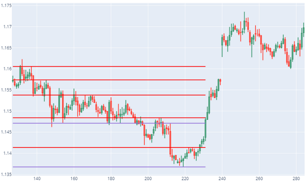
Trading solely based on the Relative Strength Index (RSI) to pinpoint overbought or oversold conditions often leads to inconsistent results. But what if there was a way to supercharge your strategy? By blending support and resistance levels with RSI to assess trend momentum, you can dramatically enhance your trade entries. This approach not only deviates from conventional techniques but also unlocks a deeper understanding of market dynamics.

In this guide, I will introduce a Python-based trading indicator that integrates these key elements. We’ll explore how to automate the detection of support and resistance levels while leveraging RSI for trend analysis. Ready to get started? Let’s dive into the step-by-step process.

Before we begin, I extend an invitation for you to join my dividend investing community. By joining, you won’t miss any crucial articles and can enhance your skills as an investor. As a bonus, you’ll receive a complimentary welcome gift: A 2024 Model Book With The Newest Trading Strategies (both Options and Dividends)

GuruFinance Insights

Step 1: Preparing the Data and Calculating RSI

First, we need to load and clean historical market data and compute the RSI.

import pandas as pd
import pandas_ta as ta

# Load the historical data
df = pd.read_csv("EURUSD_Candlestick_1_Hour_BID_04.05.2003-15.04.2023.csv")

# Remove rows where volume is zero and reset the index
df = df[df['volume'] != 0]
df.reset_index(drop=True, inplace=True)

# Check for any NA values in the data
df.isna().sum()

# Calculate the RSI with a length of 12 periods
df['RSI'] = ta.rsi(df.close, length=12)

# Display the last few rows of the dataframe to verify the calculations
df.tail()

In this foundational step, we’re working with EUR/USD hourly candlestick data. After filtering out irrelevant rows (those with zero volume), we calculate the RSI using a 12-period setting. This momentum indicator provides a measure of recent price movement strengths, setting the stage for more sophisticated analysis.

Step 2: Detecting Support and Resistance Levels

Support and resistance detection lies at the core of this strategy. Let’s define functions to identify these key levels based on candle wick behavior.

# Set the wick threshold for detecting strong rejection movements
wick_threshold = 0.0001

# Function to detect support levels
def support(df1, l, n1, n2):
if (df1.low[l-n1:l].min() < df1.low[l] or df1.low[l+1:l+n2+1].min() < df1.low[l]):
return 0
candle_body = abs(df1.open[l] - df1.close[l])
lower_wick = min(df1.open[l], df1.close[l]) - df1.low[l]
if (lower_wick > candle_body) and (lower_wick > wick_threshold):
return 1
return 0

# Function to detect resistance levels
def resistance(df1, l, n1, n2):
if (df1.high[l-n1:l].max() > df1.high[l] or df1.high[l+1:l+n2+1].max() > df1.high[l]):
return 0
candle_body = abs(df1.open[l] - df1.close[l])
upper_wick = df1.high[l] - max(df1.open[l], df1.close[l])
if (upper_wick > candle_body) and (upper_wick > wick_threshold):
return 1
return 0

Here, we calculate support and resistance levels by evaluating candle wicks relative to their bodies. A strong lower wick suggests a support level, while a pronounced upper wick points to resistance.

Step 3: Identifying Proximity to Support and Resistance

Once support and resistance levels are identified, we need to determine whether the current candle is near these levels.

# Function to identify if the current candle is close to an existing resistance level
def closeResistance(l, levels, lim, df):
if len(levels) == 0:
return 0
closest_level = min(levels, key=lambda x: abs(x - df.high[l]))
c1 = abs(df.high[l] - closest_level) <= lim
c2 = abs(max(df.open[l], df.close[l]) - closest_level) <= lim
c3 = min(df.open[l], df.close[l]) < closest_level
c4 = df.low[l] < closest_level
if (c1 or c2) and c3 and c4:
return closest_level
else:
return 0

# Function to identify if the current candle is close to an existing support level
def closeSupport(l, levels, lim, df):
if len(levels) == 0:
return 0
closest_level = min(levels, key=lambda x: abs(x - df.low[l]))
c1 = abs(df.low[l] - closest_level) <= lim
c2 = abs(min(df.open[l], df.close[l]) - closest_level) <= lim
c3 = max(df.open[l], df.close[l]) > closest_level
c4 = df.high[l] > closest_level
if (c1 or c2) and c3 and c4:
return closest_level
else:
return 0

These functions help identify when price action nears significant support or resistance levels. By incorporating proximity thresholds, we isolate relevant levels while filtering out noise.

Step 4: Confirming Price Movement Relative to Levels

To validate support or resistance strength, we examine the relationship between price action and identified levels.

# Function to check if the high prices of recent candles are below the resistance level
def is_below_resistance(l, level_backCandles, level, df):
return df.loc[l-level_backCandles:l-1, 'high'].max() < level

# Function to check if the low prices of recent candles are above the support level
def is_above_support(l, level_backCandles, level, df):
return df.loc[l-level_backCandles:l-1, 'low'].min() > level

This step provides a layer of confirmation by verifying price positions relative to historical high or low points.

Step 5: Generating Trading Signals

The magic comes alive when we bring it all together to generate actionable trading signals.

def check_candle_signal(l, n1, n2, backCandles, df):
ss = []
rr = []
# Identify support and resistance levels within the given range
for subrow in range(l - backCandles, l - n2):
if support(df, subrow, n1, n2):
ss.append(df.low[subrow])
if resistance(df, subrow, n1, n2):
rr.append(df.high[subrow])

# Merge close levels
ss = sorted(set(round(val, 5) for val in ss))
rr = sorted(set(round(val, 5) for val in rr))
# Check for signals
cR = closeResistance(l, rr, 0.00015, df)
cS = closeSupport(l, ss, 0.00015, df)
if cR and is_below_resistance(l, 6, cR, df) and df.RSI[l-1:l].min() < 45:
return 1 # Bullish Signal
elif cS and is_above_support(l, 6, cS, df) and df.RSI[l-1:l].max() > 55:
return 2 # Bearish Signal
else:
return 0 # No Signal

This function evaluates proximity to levels and trend momentum using RSI. A bullish or bearish signal is returned when conditions align, highlighting optimal trade opportunities.

Step 6: Visualizing Signals

To aid interpretation, we’ll create a chart with trading signals.

import plotly.graph_objects as go

def visualize_signals(l, n1, n2, backCandles, df):
fig = go.Figure()
dfpl = df[l-backCandles:l+n2+50]
fig.add_trace(go.Candlestick(x=dfpl.index,
open=dfpl['open'],
high=dfpl['high'],
low=dfpl['low'],
close=dfpl['close']))
fig.update_layout(title='Trading Signals', width=1000, height=800)
fig.show()

The visualization adds context by highlighting where signals are triggered on historical price data.

Final Thoughts

By combining support, resistance, and RSI within an automated framework, this strategy delivers a powerful edge. Not only can you pinpoint precise entry points, but you also gain flexibility to adapt the model with different indicators. Happy trading, and let’s code the path to success!

You can save up to 100% on a Tradingview subscription with my refer-a-friend link. When you get there, click on the Tradingview icon on the top-left of the page to get to the free plan if that’s what you want.

➡️Subscribe Me here ➡️ https://medium.com/@ayrat_murt/subscribe

I’ve got a lot to share in my upcoming blogs.

---

Automating Support&Resistance and RSI Analysis with Python was originally published in The Capital on Medium, where people are continuing the conversation by highlighting and responding to this story.